The parallel coordinate plot displays multiple y-axes, and shows the observations across several dimensions as lines. This function work well with both numeric and categorical variables at the same time after proper scaling.
geom_pcp(
  mapping = NULL,
  data = NULL,
  stat = "pcp",
  position = "identity",
  ...,
  method = "uniminmax",
  freespace = 0.1,
  boxwidth = 0,
  rugwidth = 0,
  interwidth = 1,
  resort = NULL,
  overplot = "hierarchical",
  reverse = FALSE,
  arrow = NULL,
  arrow.fill = NULL,
  lineend = "butt",
  linejoin = "round",
  na.rm = FALSE,
  show.legend = NA,
  inherit.aes = TRUE
)
Arguments
| mapping | Set of aesthetic mappings created by [aes()] or [aes_()]. If specified and `inherit.aes = TRUE` (the default), it is combined with the default mapping at the top level of the plot. You must supply `mapping` if there is no plot mapping. |
|---|---|
| data | The data to be displayed in this layer. There are three options: If `NULL`, the default, the data is inherited from the plot data as specified in the call to [ggplot()]. A `data.frame`, or other object, will override the plot data. All objects will be fortified to produce a data frame. See [fortify()] for which variables will be created. A `function` will be called with a single argument, the plot data. The return value must be a `data.frame`, and will be used as the layer data. |
| stat | The statistical transformation to use on the data for this layer, as a string. |
| position | Position adjustment, either as a string, or the result of a call to a position adjustment function. |
| ... | Other arguments passed on to [layer()]. These are often aesthetics, used to set an aesthetic to a fixed value, like `colour = "red"` or `size = 3`. They may also be parameters to the paired geom/stat. |
| method | string specifying the method that should be used for scaling the values in a parallel coordinate plot (see Details). |
| freespace | A number in 0 to 1 (excluded). The total gap space among levels within each factor variable |
| boxwidth | A number or a numeric vector (length equal to the number of factor variables) for the widths of the boxes for each factor variable |
| rugwidth | A number or a numeric vector (length equal to the number of numeric variables) for the widths of the rugs for numeric variable |
| interwidth | A number or a numeric vector (length equal to the number of variables minus 1) for the width for the lines between every neighboring variables, either a scalar or a vector. |
| resort | A integer or a integer vector to indicate the positions of vertical axes inside (can't be the boundary of) a sequence of factors. To break three or more factors into sub factor blocks, and conduct resort at the axes. Makes the plot clearer for adjacent factor variables. |
| overplot | methods used to conduct overplotting when overplotting becomes an issue. |
| reverse | reverse the plot, useful especially when you want to reverse the structure in factor blocks, i.e. to become more ordered from right to left |
| arrow | specification for arrow heads, as created by arrow() |
| arrow.fill | fill colour to use for the arrow head (if closed). NULL means use colour aesthetic |
| lineend | Line end style (round, butt, square) |
| linejoin | Line join style (round, mitre, bevel) |
| na.rm | If `FALSE`, the default, missing values are removed with a warning. If `TRUE`, missing values are silently removed. |
| show.legend | logical. Should this layer be included in the legends? `NA`, the default, includes if any aesthetics are mapped. `FALSE` never includes, and `TRUE` always includes. It can also be a named logical vector to finely select the aesthetics to display. |
| inherit.aes | If `FALSE`, overrides the default aesthetics, rather than combining with them. This is most useful for helper functions that define both data and aesthetics and shouldn't inherit behaviour from the default plot specification, e.g. [borders()]. |
Details
method is a character string that denotes how to scale the variables
in the parallel coordinate plot. Options are named in the same way as the options in `ggparcoord` (GGally):
raw: raw data used, no scaling will be done.std: univariately, subtract mean and divide by standard deviation. To get values into a [0,1] interval we use a linear transformation of f(y) = y/4+0.5.robust: univariately, subtract median and divide by median absolute deviation. To get values into a [0,1] interval we use a linear transformation of f(y) = y/4+0.5.uniminmax: univariately, scale so the minimum of the variable is zero, and the maximum is one.globalminmax: global scaling; the global maximum is mapped to 1, global minimum across the variables is mapped to 0.
overplot is a character string that denotes how to conduct overplotting
in the parallel coordinate plot. The lines from geom_pcp() are drawn according to the order they shown in your data set in default.
Note that this argument provides a framework, the order in the original data still has a role in overplotting,
especially for lines outside factor blocks(for hierarchical only), plots with resort turned on(for methods except hierarchical):
original: use the original order, first shown first drawn.hierarchical: hierarchically drawn according to the combinations of levels of factor variables, which will change according to different level structures of factor variables you provided. This was done separately for each factor block. The right most factor variables have the largest weight across a sequence of factor variables, the last level of a factor variable has the largest weight within a factor variable. Groups of lines with larger weight will be drawn on top. Lines outside of factor blocks still use the original order, which is different from other methods.smallfirst: smaller groups of lines are drawn first, placing large groups of lines on top.largefirst: larger groups of lines are drawn first, placing small groups of lines on top.
Examples
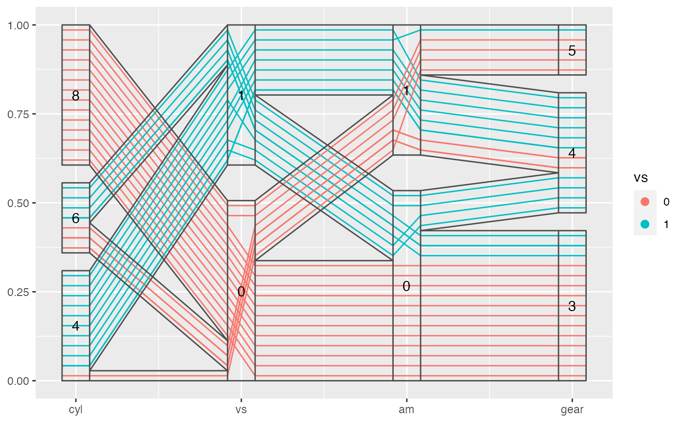
#> #>#> #> #>#> #> #>data(mtcars) mtcars %>% mutate(cyl = factor(cyl), vs = factor(vs), am = factor(am), gear = factor(gear)) %>% ggplot(aes(vars = vars(cyl, vs:gear))) + geom_pcp(aes(color = vs), boxwidth = 0.2, resort = 2:3) + geom_pcp_box(boxwidth = 0.2) + geom_pcp_band(boxwidth = 0.2, resort = 2:3) + geom_pcp_text(boxwidth = 0.2)